Application of sloppy modeling to evolution of homeothermy
According to Wikipedia, "A system is a group of interacting or interrelated elements that act according to a set of rules to form a unified whole. A system, surrounded and influenced by its environment, is described by its boundaries, structures, and purpose, and is expressed in its functioning."
For some biological systems, a single or a few gene products are so central to its functioning that, even before it was known what a gene actually was, a connection could be made between the variety of forms of a gene (the genotype) and the physical characteristic or behavior of the organism (the phenotype).
Since the first discoveries of the relationship relating DNA sequences to protein structure and functioning, many biological systems have been modeled at the molecular level. These models often become more and more complex as new experimental observations are sought to be included. Seemingly contradictory models may emerge if different sets of observations are used in their construction.
I think a systems analytic approach called sloppy modeling may be useful in understanding how homeothermy evolved. Sethna and his colleagues (Guntenkunst et al. 2007a, 2007b, Daniels et al. 2008, see also https://sethna.lassp.cornell.edu/Sloppy/) analyzed many biological systems for which models have been proposed to explain some type of behavior, either at the single cell level, for in vitro studies with cell extracts or purified components, or of developmental process of the organism. Each particular model consisted of several proposed components (macro-molecules such as proteins or DNA and various small molecules) and proposed equations whose variable parameters described the actions and interactions of the components. The models also would also contain fixed parameters describing the environment in which the action would occur.
In section 2 I will discuss the one example which first interested me in sloppy modeling and in section 3 discuss possible implications to the evolution of hoeothermy. However, there are several caveats that would seemingly make this exampe irrelevant to this exploration:
It concerns the temperature-compensated behavior in vitro of a protein (KaiC) in a procaryotic organism, seemingly remote conceptionally from how mammalian evolution.
It is, to my knowledge, the only biological systems to which this kind of analysis has applied to understand behavior over a range of temperatures.
Since this analysis was published in 2008, much more has been learned about this protein on the molecular level. An updated analysis might reach different conclusions than for the simpler model.
Despite these reservations, I think these techniques have two important advantages that could be useful here. They appear to be able to point to which components of a system are most important to any particular behavior. They also provide a means revealing levels of organization intermediate between DNA sequence (genotype) and organismal behavior (phenotype).
In the last several years, knowledge of the KaiC system has greatly progressed. including knowledge of the structures of the various configurations of the protein down to the angstrom level. This includes mutant genotypes and how they affect behavior, particularly as temperature changes. The recent success of AI in predicting folding of proteins based of their amino acid sequences suggest that it may soon be possible to more accurately predict kinetic parameters from genotype.
In section 4 I will discuss the current understanding of sloppy modeling, which has been applied to many other fields outside of biology. In discussing this broader application, Trunstrum et al, (2015) discussed the aptness of the techniques to understanding how biological systems can be both robust and evolvable, and discuss the original analysis of KaiC as an example,
1. Sloppy modeling techniques
For a particular model, the equations would have n variable parameters (Θ1, Θ2, ...,Θn). Any set of estimates of these parameters can be considered to be a vector (Θ) in an n-dimensional space, which they called the chemotype space. The experimental data of the behavior of the system consisted of the initial concentrations of the measured component and m subsequent measurements (di) at various times (ti) of the concentrations of some of the components. This observed behavior can be considered to be a vector in a m dimensional space, which they call the dynatype space, since it encapsulates the the observed dynamic behavior. Since the properties of the macromolecules of any particular organism are determined (at least in part) by the nucleotide sequences of genes, it can be seen that chemotypes and dynatypes are organizational levels between the genotype and higher levels of organization resulting in observed phenotypes.
For each system and model, they ran simulations varying all the parameters over a wide range of possible values. For each parameter set, they calculated a sum of the squares between the predicted (yi) and observed data points, the so-called cost equation:
They then determined where all the points were in chemotype space for parameter sets where this sum was less than some value. I will call these "success" sets.

For all the systems they studied, if the parameter values were plotted for all the successful sets, the range of values of some parameters were small, but range of values for other parameters were up to a few orders of magnitude wider. It was useful to plot these successful sets on log axes.
They found that almost all success sets lay within a hyper-ellipsoid in this (log) chemotype space. An n-dimensional hyper-ellipsoid is a shape whose boundaries in any plane is an ellipse. It can be delineated by its center point and n orthogonal axes and their corresponding diameters. For all the systems they studied, the values of these diameters were spread over a wide range. They called this property "sloppiness," A direction in n-space with a small diameter is called "stiff" and a direction with a large diameter is called "sloppy."
One interpretation of sloppiness is that only a small fraction of the parameters or, as we will see, combinations of parameters, need to be known with some degree of certainty for the model to reasonably replicate behavior of the system. Since the first application of this kind of analysis, sloppiness has been observed for a number of models of system in other fields, such as physics and biology. Section 4 will discuss other interpretations of sloppiness.
To get an idea of what the stiffest directions are, it is usefui to relabel the parameters so the two with the least variability are now labeled 1 and 2. The figure at right illustrates what is typically found. The yellow circles show the successful sets projected onto the Θ1, Θ2 plane. The ellipse encompasses these points. The other lines outside the ellipse (partially) show what the boundaries of the ellipse would be if the value of the cost function for a set to be successful was made progressively larger.
For the hypothetical case presented, the stiffest direction is from the upper left corner to the lower right corner. The center of the ellipse would be near that for the set of parameters with the lowest cost function. Moving a small distance in chemotype space in either way along the stiff would reach parameter sets which would no longer be successful.
The next stiffest direction is along an axis from the lower left to the upper right, where the change in log Θ1 is approximately equal to the change in log Θ2. As long as a change in parameters was in this direction, a larger change could occur before leaving the success region, as compared to changes in the stiffest direction.
What about changes in a very sloppy direction. These can be very large because any change in one of parameters associated with that direction can be compensated for by small changes in the other parameters.

2. Sloppy modeling of a temperature-compensated system
The cyanobacteria (blue-green "algae") are the simplest organisms to exhibit circadian rhythms. As in other organisms, light triggers an oscillation with a period around 24 hours in the transcription and translation of certain genes. Observations by Xu et al. (2000) on the cyanobacterium Synechococus elongatus indicate that the clock mechanism continues to oscillate even when the cells are transferred to the dark, which inhibits almost all transcription.
Oscillations of the messenger RNAs for the proteins, KaiA, KaiB, and KaiC occur during continous light exposure and mutations in any of these genes abolishes the circadian rhythm. When cells were exposed to light for 12 hours, by which time the concentration of Kai messenger RNAs had reached a peak, then placed in the dark for various times (2-42 hours) before returning to the light, when the mRNA oscillation resumed it had the same phase as for the cells that were continullay in the light. For example, the peaks in mRNA concentration occurred around 36 (if the light was restored before), 60, or 84 hours.
The KaiC protein can be phosphorylated (a phosphate group co-valiantly linked). Mutations of the site of phosphorylation can abolish the circadian rhythym (Xu et al. 2004). Tomita et al. (2004) measured phosphorylation levels of cells kept in the dark and found that it oscillated with a period of about 24 hours regardless of whether the temperature was 25, 30, or 30C.
A cycle of phosphorylation and dephosphorylation of KaiC occurs in vitro for KaiC when supplied with ATP in the presence of KaiA and KaiB, which again continues with a cycle near 24 hours even in dark, and for temperatures ranging from 25 to 35 C. Since the rates of chemical reactions generally increase exponentially with increases in temperatures, how does this compensation for changes in temperature occur?
Behavior which does not change with temperature over this range is observed in an even simpler in vitro system.
It was known that KaiC could phosphorylate itself, but that the rate was much higher in the presence of KaiA. Tomita studied in vitro systems consisting of purified KaiC and KaiA or just KaiC, along with ATP (the source of phosphates), a buffer and salts. Initially about 0.4 of the phosphoryation sites on the purified KaiC were phosphorylated. For KaiC alone It was found that the level of phosphorylation increased slightly in the first 30 minutes, then decreased steadily for the remainder of a 6 hour period, and the rate of decrease was the similar at the three temperatures(top part of figure at right). When KaiA was also present, the phorphorylation increased steadily, reaching about 0.8, again at the about the same rate at the three temperatures.
Tomita presented the model at right to explain how the phosphorylation cycle of KaiC could be maintained in the dark without requiring continuing transcription and translation. Binding of KaiA to KaiC would cause phosphorylation of KaiC. This would continue until KaiB limited this activity. At this point phosphorylated KaiC would start to de-phosphorylate. They attributed the subsequent reinitiation of phosphorylation to some unknown process related to changes in the internal state of KaiC dependent on the level of phosphorylation.
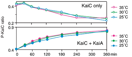
Figure 3d of Tomita et al. (2004)

Daniels et al.(2008) analyzed the data for phosphorylation of KaiC alone using a model developed by van Zon et al. (2007), which is described in detail ion page 2A. Two key features of this model was that it incorporated two features of KaiC, it can switch between two allosteric (shape) configurations and is always found as an aggregate of 6 monomers (a hexamer).
Figure 4 of Tomita et al. (2004)
2A. von Zon model
It was known that KaiC has two sites at which it could be phosphorylated, but van Zan they chose to assume one site. Also in 2007, two papers were published (Nishiwaki et al. (2007) and Rust et al. (2007)) that presented evidence that sequential phosphorylation of both sites and subsequent dephosphorylation of both sites is a requirement for oscillation. Neither paper considered the allosteric changes mentioned above. Understanding the temperature compensation of KaiC cycling would certainly benefit from an updated sloppy model including these and more recent findings. Recent understanding of the 3D structures of the hexamer (see at different stages of the cycle using x-ray crystallography) (Furuike et al. 2022) and predictions of effects of phosphorylation on protein folding would benefit such a re-examination. This is discussed in detail on page 2B.
2B. Updated KaiC model
3. Homeothermy- robustness and evolvability
Despite the limitations of the van Zon discussed above, I think the analysis by Danels et al. may be relevant to the evolution of homeothermy. The figure below shows the results with all the successful parameter sets projected onto the plane of the two parameters with the least variation (out of 36 parameters)

It can be seen that at single temperatures, the diameter of the ellipsoid in the stiffest direction is small, even compared to the diameter in the second stiffest direction. Also, many of the pairs of two parameters would be the same for sets of successful parameters at both 30 and 35 C. However, many of these parameter sets would not provide a good fit to the data at 25 C.
Seemingly contrary to this, some of the parameter combinations that were judged successful for all three temperatures (black points) would not be judged successful at 25 C. However, it must be remembered that in the definition of the cost function, the sum of the squared residuals is divided by the number of measurements, so the threshold for successful fits is related to the same "average" goodness over all the data points.
Keeping in mind the vast majority of mutations are not lethal or render the organism sterile, how might a cumulation of mutational changes effect the behavior of this model system. Mutations that moved the parameters in the stiffest direction only a small distance in chemotype space would be expected to be selected against if the system that has to function reasonably well over a range of temperatures. Such conditions require the system to be precise, only a limited range of parameters can be successful.
In contrast, if success were required only at a single temperature, over time mutations that changed the parameters along the second stiffest direction could move a larger distance in chemotype space, because in the population there would be other mutations that made suitable (small) changes in the sloppier parameters.
S elongatus strains appear to be adapted wide range of environmental conditions, from temperate to tropical climates to hot springs. The strain used in the above temperature compensation studies, PCC 7942, was isolated prior to 1973 at California State University at San Francisco and added to the Pasteur Culture Collection in 1979, so presumably was originally adapted to a range of temperate temperatures.
Could the slow change from ectothermic to homeothermic behavior resulted in many systems becoming less susceptible to mutational change (increased robustness), and for their components individually to act more precisely and interact with other systems (increased complexity, novelty, and evolvability)? Once this newer behavior was established, it likely would lessen the range of temperature fluctuations that could be tolerated, as suggested by the findings in Exploration 1)
4. Later developments in sloppy modeling
The original developers of sloppy modeling techniques seem to have been mainly biophysicists and systems analysts. I think their application of these techniques to the concepts of chemotype and dynatype spaces should have interested many biologists. However, this does not seem to be the case, perhaps because of mathematics involved and the large computational resources required. Subsequently, the techniques have been found to be useful in many other fields, such as physics and economics, where computational techniques are routinely used.
There appears to be two attitudes towards the concept of sloppiness. Some think it is a general feature of reality that allows even complex systems to be (at least partially) understood in terms of the properties of just some of their components. Others attribute sloppiness to the uncertainty to be expected when there is not sufficient relevant data to analyze an overly complex model.
Whatever the case, techniques have been developed to simplify proposed models. Transtrum and Qiu (2014) developed a procedure they called Manifold Boundary Approximation Method (MBAM) which they applied to a model involving two extracellular signals interacting through a network of proteins to activate the Erk1/2 proteins. This model had 19 components, 29 differential equations, and 48 parameters. They were able to reduce this to a model that fit the data just as well with 9 components, 6 differential equations and 12 parameters. Some components were eliminated as irrelevant or their number reduced by combined actions being coalesced into a single parameter.
The reverse process may be possible. If there is some components shared by two distinct processes, simplified models of each process could be derived and then studied to see what limitations are placed on the ranges of successful sets of parameters by requiring both processes proceed properly.
Incidentally, of interest for topics of this site, the Erk1 and Erk2 proteins play prominent roles in cellular proliferation and inhibition of programmed cell death (apoptosis). They play a critical role during the phylotypic period of embryonic development. Mice lacking Erk1 usually do not survive gestation. Mutations of the genes of this Erk1/2 pathway are frequently found in several types of cancers.
For axial patterning at the beginning of the phylotypic period, Erk1 activation in the presomitic mesoderm (by the double phosphorylation of Erk1 ppErk),) in the posterior end of the embryo results from the extracellular release of fibroblastic growth factor 3 (fgf8). This keeps these cells in a “stem cell-like” proliferative state. As these cells move anteriorly, they enter a region of lowered fgf3, divide more slowly and begin differentiating into somites (the precursors of vertebrae and muscles).
Two phosphatases (DUSP4 and DUSP6) act to shapen the gradient of ppERK at the point of somite formation, assuring that the have well-defined boundaries (only a few cells thick). This is reminiscent of the interplay of double-phosphorylation and dephosphorylation in producing a precise circadian clock in blue-green algai, discussed in sections 1 and 2. The Erk system is discussed further in parts 3 and 4 of Background 9 in connection to developmental scaling.