Another Cost of Fire
Robustness, Evolvability, and Complexity
One impetus to construct this site was the reading "The Fires of Life: the evolution endothermy in birds and mammals" by the late Barry Lovegrove. Much of the book detailed how the benefits of increased energy production (through physiological and anatomical changes) came at the cost of needing to consume more food. Endothermy allowed entry into hostile environments in which the availability of food might be sporadic or unpredictable. Endotherms became more robust in some ways but more vulnerable in others,
In the slow evolution from endothermy to homeothermy in mammals, it seems likely that many of the biological systems would have in some ways become simpler, since they would no longer have to function properly over a range of temperatures, no longer needing to be robust to this environmental change. Did the decreased necessity for this kind of robustness allow greater evolvability? Did the changes this allowed in turn make organisms less robust in other ways?
What would be the best organisms and tools to look for such changes?
Almost all biological processes occur faster at higher temperatures. Most enzymatic reactions have a Q10 (the fold increase in rate for a 10C increase) of 2-3. As discussed previously, timing of different developmental events is probably the most complicated from the gastrula through the pharyngula stages. The three vertebrate organism that have been most extensively studied in these periods are the zebrafish, the chicken, and the mouse. The zebrafish are, of course, poikilothermic. In the wild zebrafish are found in the rivers of the Indian subcontinent, but mating and egg-laying occur in shallow flooded ponds and rice fields where a temperature range of over 14C has been observed (Engezar et al. 2007). Shroeter et al. (2008) observed no difference in somite (precursors of segmented metadermal tissues) size between 21.4 and 31C, even though somite formation occurred 3 times faster at the higher temperature. Chickens are likely less homeothermic than mice. The timing of events in this period will be the subject of Exploration 3. In this section, I will concentrate in finding tools to use in that exploration.
According to Wikipedia, "A system is a group of interacting or interrelated elements that act according to a set of rules to form a unified whole. A system, surrounded and influenced by its environment, is described by its boundaries, structures, and purpose, and is expressed in its functioning."
For some biological systems, a single or a few gene products are so central to its functioning that, even before it was known what a gene actually was, a connection could be made between the variety of forms (alleles) of a gene (the genotype) and the physical characteristic or behavior of the organism (the phenotype).
Sethna and his colleagues (Guntenkunst et al. 2007a, 2007b, Daniels et al. 2008) developed a methodology for analyzing systems in terms of two different levels of biological organization intermediate between the genotype and the organismal phenotype. They analyzed many biological systems for which models have been proposed to explain their dynamical behavior. Each system is characterized at any particular time by the concentrations of its components, which may be various small molecules and various macromolecules in different internal states. Each model system consisted of equations that describe their rates of change of the components.
I became interested in this methodology for three reasons. It addresses both the robustness of genotypes against mutational change and the capacity of a system to change (evolve) without affecting critical functions. For systems in which multiple genes determine an organismal phenotype, the methodology provides a way of judging their relative importance. Finally, this approach might be useful in understanding what new adaptations could have been possible as homeothermy shrank the range of temperatures over which a system must function properly.
I don't know if such a study has ever been attempted. A starting point would be understanding how systems achieve temperature compensation. To my knowledge, this methodology has only been applied to one such system, part of the circadian clock mechanism in a blue-green algae (Daniels et al. 2008). I will discuss this system briefly and then in more detail in 3 additional sections. Since that study, many more details of this system have been learned, down to the level of the positioning of atoms in the protein involved. New insights have also been learned about the interpretation of the methodology.
Sethna et al. determined how well the observed dynamic behavior of a system could be simulated by a proposed model. The behavior to be modeled consisted of the concentrations of some of the components measured at various times under a particular set of experimental conditions with a total of m measurements. This was called the dynatype. A particular set of the n values of the parameters (θ1..θn) of the model equations is called a chemotype. For a particular chemotype, starting with the initial conditions, they could calculate the predicted values of the data points, The "cost value function" could then be calucuated as the sum of the squares of the difference between the predicted and observed values. They did this for a for a large number of combinations of parameters to determine which chemotype best reproduced the dynatype, i.e., the chemotype with the smallest cost value.
They were interested in how much changing the values of the parameters in the vicinity of best-fit chemotype would affect the goodness of fit. They determined which chemotypes had cost values somewhat higher than the best fit value. I will call these the good-fit chemotypes. When all the good fit combinations were plotted in n-dimensional parameter space, the region containing them could be approximated by a hyperellipsoid. As such, if all the good fit parameters for any two dimensions are plotted, almost all the points fall within an ellipse. For some parameters there was only a limited range of values for good fit chemotypes.
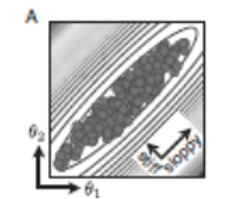
The figure at right shows such a typical ellipse (with the two parameters with the most limited range relabeled as 1 and 2). It can be seen that for particular value θ1, only a narrow range of θ2 values are still in the good fit region, and vice versa. The narrowest diameter is along a line with a slope of around -1. This direction in parameter space is said to be "stiff." In the direction at right angles to the stiff direction the diameter is considerably larger; this direction is said to be "sloppier". It can be seen that even if parameter 1 changed a value in the lower part of its range, some set of values could still be found that produced a good fit, but only if particular changes also occurred in parameter 2 and also in some of the other n-2 parameters.
An n-dimensional hyperellipsoid is defined by its central point and n diameters along the n orthogonal directions of its axes. For all the systems, models, and data sets studied, the resulting set of good-fit diameters had a large variation in their relative ranges, frequently by more than an order of magnitude. Thus, many of the axis directions are truly very sloppy, much more than the sloppy direction shown in the above figure. This raises the question if some of the extreme parameter values are realistic. The figure below addresses this question. It illustrates a system with only two parameters, and the good fit sets of parameters lie within an ellipse in chemotype space with one stiff direction and one sloppy direction.
The actual chemotype values in an organism depend, in part, on the underlying genotype, and are thus subject to change by mutation. Suppose that the initial chemotype of a system is near the best fit chemotype. The circle in chemotype space of radius δ in the figure represents the possible changes in chemotype due to mutations. If the actual chemotype were near the best fit chemotype it can be seen that mutations (occurring in a single generation) that change the chemotype in the sloppy direction would still be a good fit, but only if there was no more than a small shift in the stiff direction. Conversely, a larger portion of mutations that produced changes in a stiff direction would no longer produce a good fit. If the particular behavior affected reproductive fitness, then we would be justified in discussing fitness, and not just a good fit. So, after several generations, the actual chemotype might "drift" some distance in a sloppy direction. But the farther away one moves in a sloppy direction, the smaller the range of good fit values is in the stricter direction(s). An individual to end up with a chemotype at extreme in a very sloppy direction, its ancestors would have been extremely "lucky" to have escaped fitness-reducing mutations that produced changes of chemotype in strict directions. In a population of individuals we would expect clustering around the best fit chemotype, but with more variation in sloppy directions than in strict directions.

It can be seen that systems with some strict directions will be less robust against mutational harm than a system with fewer or less strict directions. Daniels et al. (2008) developed a crude estimation of the mutational robustness. For each chemotype, there is a corresponding dynatype consisting of m data points, each being the concentration of a component predicted at each measurement time. The shaded region in dynatype space is meant to enclose all the dynatypes for the good-fit chemotypes. It is depicted as a sphere with a radius of ε. This would actually be the case if m=3 and for each of the data points the data points for the set of good-fit chemotypes had the same range of values. Whether the assumption that this region is a m-dimensional hypersphere will be discussed later.
The dataspace ellipse depicted is meant to represent the volume enclosing all the dynatypes representing the possible chemotypes after mutations. Even if m were as low as 3, this region would not be planar as depicted. For a two-parameter system it would be a ribbon-like structure twisting and turning in 3-dimensional space. The length of the ribbon corresponds to the stiff chemotype direction and the width to the sloppy direction. As depicted here, this width is less than ε. Mutations that solely changed the chemotype in this direction would still give good fit chemotypes. In contrast, if one of the radius of the good-fit hyperellipsoid is less than some (unknowable) amount, we would expect some mutations that produce chemotypes that would produce a bad fit, which might be associated with reduced fitness. Although rather crude, I think this principle can be of use in understanding some consequences of homeothermy.
The radii of the best fit hyperellipsoid can be calculated by the "curvatures" of the cost function in the vicinity of the best fit chemotype. The best fit chemotype is defined as that position in chemotype space where the cost function is a minimum. For a two-dimensional curve described as y being some function of x, y=f(x), if the function is at minimum for some value of x, x(min),then the first derivative (slope) of the function at this point is 0. The second derivative of the function at x(min) is the curvature. For a point x in the vicinity of x(min), the function can be approximated as f(x)= f(x(min)) + (curvature X (the square of (x-x(min)))/2.
For an n-dimensional cost function, the minimum is at the best fit set of parameters, and the n by n matrix, called the Hessian, with the second derivative of the cost function with respect to the ith and jth parameters being the i,j entry. The eigenvectors of this matrix will point in the n directions of the good fit hyper-ellipsoid axes. The n eigenvalues are (inversely) related to square of the radii along each axis, i.e., if the radius in the ith direction is smallest(the strictest direction), the ith eigenvalue is large and for progressively larger radii, the corresponding eigenvalues are smaller and smaller.
The figure at right shows eigenvalues determined in a study (Daniels et al. 2008) of the in vitro behavior of the KaiC protein, the central component of the circadian rhythm system of a blue-green algae. It was known that in vivo the phosphorylation (covalent attachment of a phosphate) level controlled which genes were expressed at different times of the night and day and varied with the same period of around 24 hours whether the temperature was 25, 30, or 35°C. In an in vitro system with only two components, purified KaiC and ATP(as a source of phosphate), the level of phosphorylation initially increased then decreased for the remainder of the experiment. The behavior was the same at the three temperatures, despite all the rates of change between states of the system expected to increase as the temperature increased.
The buttons below go to the pages describing the details of the formulation of a model for this system consistent with other observations of this system and the application of the sloppy system analysis.

In the figure the horizontal lines farthest to the right are the eigenvalues for a model that is required to simulate the (similar) observed behavior at the three temperatures. As for all the systems to which this methodology has been applied, the eigenvalues are spread over a wide range, which is the definition of a sloppy system. There were 36 parameters in the model used. It can be seen that only a handful of these parameters are at all critical to fitting the data.
In contrast, the lines on the left are the eigenvalues for a model that is only required to produce a good fit the observed behavior at a single temperature. There are only three relatively large eigenvalues (three strict directions), while all the others are much lower by orders of magnitude. It can be seen that the largest eigenvalue for the three-temperature fit is larger than that for the single-temperature fit, as it is for the second and third largest eigenvalues. Larger eigenvalues would generally be expected to be associated with less robustness to mutation affecting function. Even though we can't say what the critical eigenvalue would be that below which we would not expect any mutations to affect function, the results suggest that the reduction in range of temperatures over which systems must function brought about by homeothermy resulted in greater robustness agains mutational change.
The mathematical used to study each system is described in detail in Gutenkunst et al. (2007). For every set of parameters (θ1..θn) they ran a computer simulation of the model and recorded the predicted phosphorylation at each time data had been recorded. For each data point they then calculated the square of the difference in phosphorylation between the experimental data and the model prediction and added this up for all the data points. So this was just a standard sum of squares estimation to judge the goodness of the fit. I will call the sets of parameters that had a sum of squares less than some value a success, though the original authors did not use this term.
Every combination of parameters which produced success was plotted as a point in n-dimensional space of the log of each parameter. For this system, and all the other biological systems Gutenkunst studied, the success region was found to be reasonably approximated by an n-dimensional hyper-ellipsoid. It is typically found that a few parameters cannot vary much without precluding success, and thus their values are critical, while most of the other parameters can vary considerably more without affecting success.
They typically would designate the two most critical parameters as θ1and θ2. The figure at right shows what is typically observed: Most of the successful points (circles) from varying θ1and θ2 lie within an ellipse. The other lines around the ellipse represent ellipses that would be obtained if the range for success is increasingly made larger.
In the illustrative example shown at right, if we "move" in parameter space so that θ1 increases while θ2 decreases (or vice versa) the sum of squares of successful parameter sets changes rapidly with distance. This direction is described as being "stiff." In contrast, if θ1and θ2 change together, the output changes considerably slower. This direction would be "sloppier." In reality, this direct is actually rather stiff. The sum of squares changes even more slowly if we had moved in any other direction involving the other n-2 parameters.
The positioning and shape of the "success" hyper-ellipsoid can be described by it's n (orthogonal) axes and their corresponding diameters. The axis with the smallest diameter is oriented in the stiffest direction.
Several remarkable findings were found for all the systems studied by this technique. There are only a few relatively stiff directions. In most systems the stiffest direction did not align completely with movement in the direction of a single parameter (see Figure 1C of Gutenkunst et al. (2007)0. If this were the case of a plot of success points on a log(θ1)log(θ2) graph would have the success ellipse oriented vertically. Instead, for the critical parameters, changing one parameter would preclude success unless there were compensating changes in a few other parameters. In the figure above, a small change if θ1 would preclude success is it were not accompanied by a particular change in θ2.
For all of the biological models studied, the diameters along the axis of the hyper-ellipsoid are spread out over a large range. They called this property sloppiness. This strongly suggests that sloppiness is also a property of the biological systems that the models mimic. It should be emphasized that just because a very wide variety of sets of model parameters produce success (if only "on paper"), most of these sets could not actually be substantiated in a set of actual components. The parameters of the system associated with a particular macromolecule depend (although not entirely) on the sequence of the gene from which it derives, its genotype.
The parameters associated with an actual system have been called its chemotype. The behavior of the system can be thought of as a point in "behavior space," the behavior called its dynatype It has been suggested that all feasible dynatypes would lie on a "hyper-ribbon" in this space and thus also have characteristics of sloppiness. I real ribbon in 3-dimensional space is characterized by three sizes, its thickness (small, the stiff dimension), its width (larger, thus sloppier), and its length (large, thus sloppiest.). There are likely more layers of complexity when we consider the myriad interactions of systems to produce the behavior observed in whole organisms.
In a population of organisms, large difference of overall behavior between individuals are called phenotypes. It seems amazing how often we can relate these phenotypes to a few different genotypes and understand them in terms of simple Mendelian concepts such as homozygosity, heterozygosity, dominance, recessive, etc.
In contrast to sloppy systems, in a precise system, movement by small distances in most directions in parameter space would move the system out of the success region. If biological systems were too precise, they would be prone to failure because many of mutations occurring in genes coding for components of the system would change the parameters enough to preclude functioning successfully. Sloppiness thus confers robustness. In another section, I argue that homeothermy allows more precision in an organism's systems, and also allows increasing complexity in the interactions of those systems.